Over the last two decades, facilities have developed an array of asset management programs to improve compliance and overall risk management, but they largely remain in a state of reactivity. Or, at times, the list of activities can be overwhelming and make it hard to prioritize what to do first. Facilities are constantly working in defense mode rather than offense, with never ending piles of work orders stacking up. But what if facilities were able to predict the bad and mitigate it before it happened?
The TBA is highly inefficient because it often results in large amounts of resources being spent disproportionally to the risk of each asset. These dated practices also do little to encourage the operator to become deeply educated on their units, systems, or the interdependent effects of operating practices on different types of equipment. A TBA is overly conservative and is often wasting time and money inspecting assets that do not need it or sometimes not inspecting often enough. An RBI program considers past events, current conditions, and can help predict the best future operating practices and their effects on the integrity of the equipment.
Reliability Centered Maintenance (RCM) Programs
On the non-fixed equipment side, RCM has traditionally been thought of as a one-time study that follows a systematic set of questions called a Failure Modes and Effects Analysis (FMEA) and identifies a set of tasks to mitigate these failure modes. Equipment criticality is defined based on the consequence of these failures.
An enhancement to the traditional RCM methods was the introduction of risk into the analysis. Risk is defined as the product of the Probability of Failure (POF) X Consequence of Failure (COF). Most RCM analyses in the last two decades have incorporated probability into the analysis to define equipment criticality by developing risk matrices for various criteria such as safety, environmental impact, production loss, financial impact, and reputation impact.
There are some limitations to these methods that cannot be ignored. First, these programs are only as good as the data you put into them. RBI and RCM models are static and require constant evergreening in order to produce accurate results. Special emphasis programs such as traditional CML Optimization methods, often require adding more CMLs but rarely evaluate if any CMLs can be removed. Why do we often still feel like we are in a reactive mode with these traditional proactive methods?
Overcoming Model Limitations with QRO
Quantitative Reliability Optimization (QRO) brings a new approach to reliability—the first model to incorporate both fixed and non-fixed assets into one analysis—and can optimize tasks for an entire facility based on how they all operate together. QRO demonstrates an approach that ensures all reliability decisions have strong financial backing at a plant level. Because of this, QRO can forecast which assets drive changes, associated costs, and risks for both today and in the future. It can also forecast which assets drive changes, associated costs, and risks. This forecast is powered by individual assets in the model singularly shaped off individual data points to roll up to a System Model.
A System Model is where a reliability block diagram is built of all the assets in your facility. It defines the relationships among your assets, such as whether they are parallel or in series or whether there is a percentage throughput that needs to happen through them. They can then be visualized much like a Process Flow Diagram (PFD) for a Reliability and Maintainability (RAM) analysis, so there is a calculated model that is continuously being updated with how each asset’s uptime affects the system or plant’s uptime. From there, you can drill down on each asset and look at economic risk or health and safety (HSE) risk.
Using the Data You Already Have
QRO is powered by the data you already have from your Inspection Data Management Software (IDMS), Computerized Maintenance Management System (CMMS), data historians, vibration analysis, and other sources through easy imports or software connectors. QRO is not meant to replace those tools; instead, it harnesses and leverages all that data together in one location and one model.
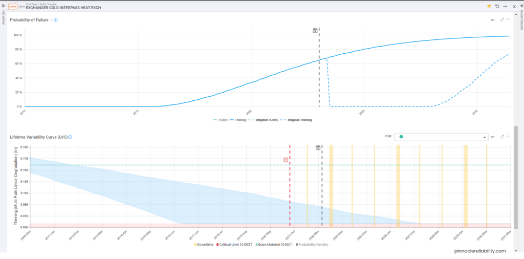
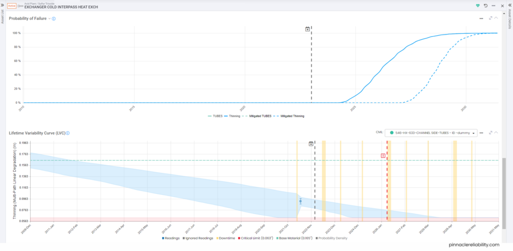
But what if you don’t think you have enough data to build a program? You don’t need decades of data to begin a QRO program. Using SME as your baseline data point and now gather a new data point. Just by adding one data point you can now extend the forecast failure window by five years.
Image 2: Same exchanger as Image 1 with additional data from an Eddy current inspection
Example
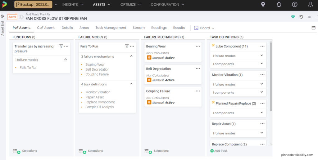
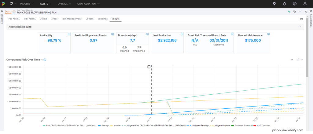
QRO harnesses the power of data science to supplement facility data. The example below walks through an Asset Risk Analysis (ARA) for an individual fan. The fan is broken down into a few major components, the bearings and the impeller, but it could be broken down into more complexity if chosen. An FMEA was set up with selected failure modes, what is driving those failure modes, and within those failure modes, how are they going to fail from a modeling standpoint.
Image 3: Example FMEA dashboard for piece of equipment
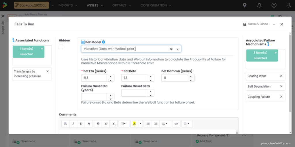
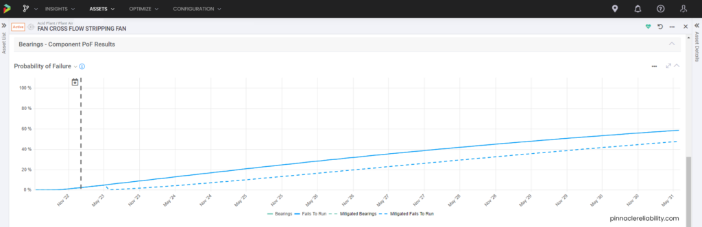
Image 4: Example of in depth look at a POF model
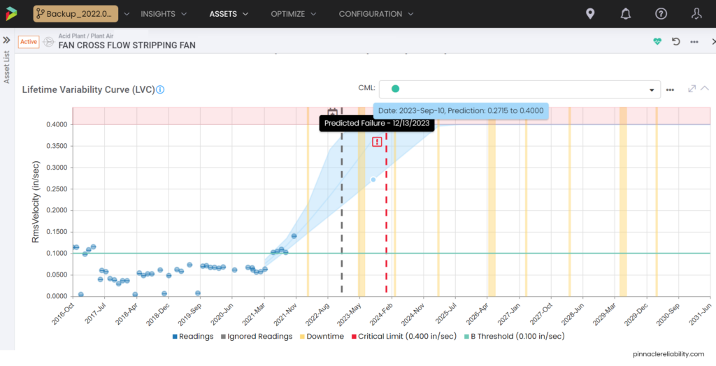
Weibull analysis parameters priors are set up and require condition monitoring from vibration feeding into this failure mode. So now it can constantly update for a live risk and level of uncertainty. Now we need to understand the impact of that failure, which, in this case, is a one-day outage equaling about $3M in lost production. So, then the question is, “how do I know when this will break beyond just the Weibull parameters I have set up?” The model attaches vibration monitoring readings and plots the results onto a Lifetime Variability Curve (LVC). The LVC, based on Bayesian statistical models, can forecast the point we expect the earliest onset of damage, the most likely failure point, and the latest possible failure point.
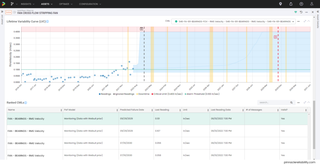
Image 5: Example LVC showing predicted failure after next planned shutdown
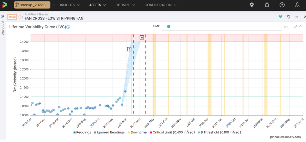
Each one of the bearings has its own criteria for failure and its own calculations for its forecast. One shows that there will be a failure prior to the next shutdown, so what do you do?
Image 6: Example LVC showing predicted failure prior to next planned shutdown
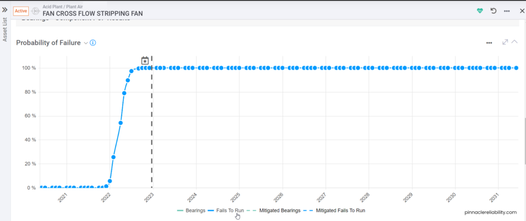
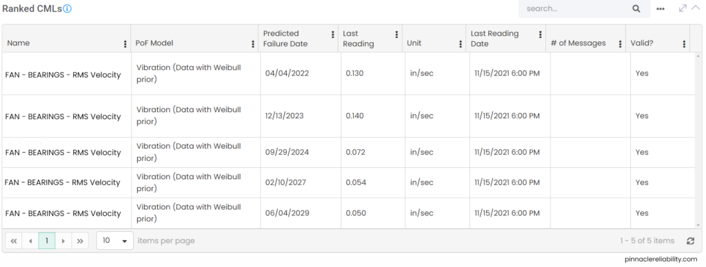
View the tasks planned out and work history pulled from the CMMS for this component, and you can now start to plan out new tasks to help mitigate this risk. When you go to the results tab and understand that the worst actor CML (here the Fan’s Onboard Vertical Vibration sensor) in this vibration analysis funnels into a risk profile that shoots up from a 0% to 100% chance of failure in only a couple of months span that guarantees a failure.
Image 7: Example POF curve if equipment is let run to fail
Image 8: Example of worst actor CML list
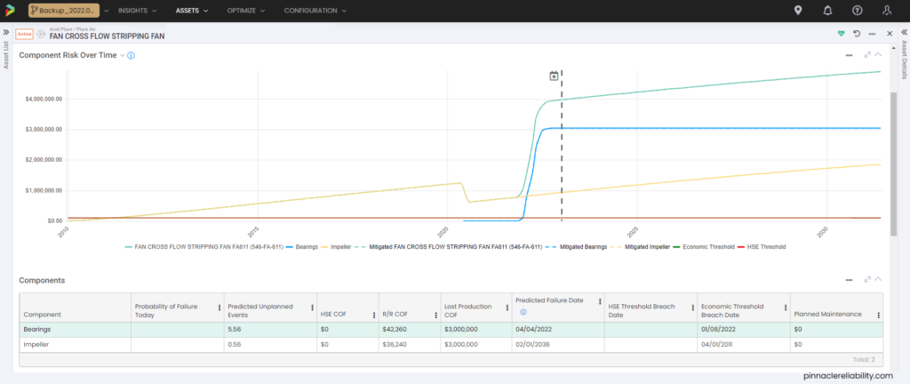
Image 9: Example of overall asset risk without any mitigation
This early failure means that we need to intervene. So, in this actual scenario with the client, that is what we did. We intervened by saying, “let’s do some maintenance now, but also plan out some more comprehensive repair tasks.” Now let’s fast forward a bit, and the image below shows what those forecasts look like after repairing the bearing component, plus one new vibration reading after installation, and see how much that LVC failure range is widened into the future, expected lifespan is being extended, and the effect on the POF distribution curve.
Image 10: New LVC for asset after repairing the bearing component and an additional vibration reading.
Image 11: New POF curve after repairing the bearing component and an additional vibration reading.
This mitigation hasn’t solved all the problems with this asset; we still need to plan the major repair/replace tasks for the next shutdown. Note that the blue line for the bearings component restarts after the May 2022 repair, but the impeller risk remains high on the solid yellow line, with the two combining to make the overall green asset risk line. Both components’ Mitigated Risk (dashed lines) drop in May 2023, given the added plan for full asset repair/replace task during next year’s shutdown.
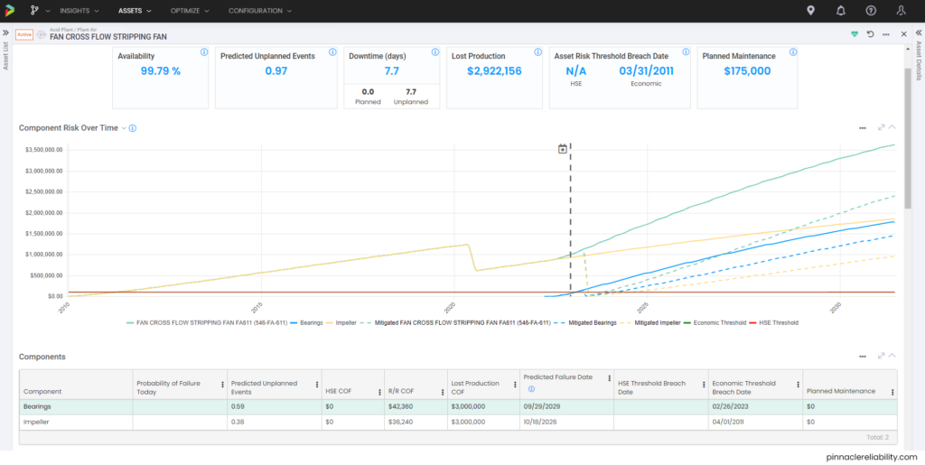
Image 12: Example of risk reset after repairing bearing component
Image 13: Example of risk reset after repairing bearing component
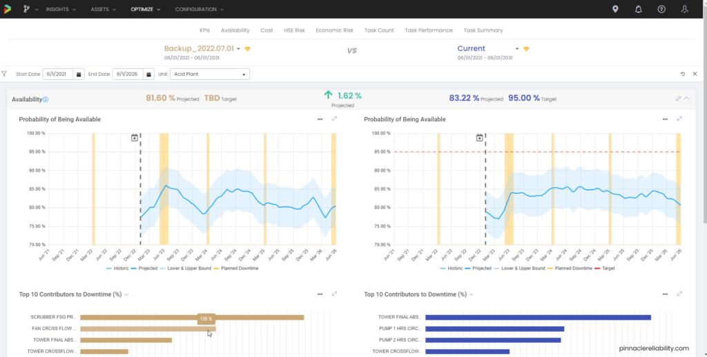
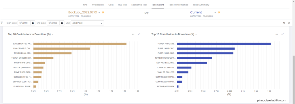
To add additional economic justification to say these tasks were worthwhile, you can build out what-if scenarios and constrain different parameters around HSE, economic risk thresholds, and availability impacts. This allows you to make an A to B comparison with your plans and recognize what it was all worth. For our fan scenario, the overall plant availability has increased by over 1.6%. You can also see that before the repair, the fan was the number two worst actor, and after the repair, it dropped off from the top ten worst actor list.
Image 14: Example of overall scenario comparison, showcasing facility availability
*Note: The fan in this example has completely dropped off the bad actors list, but also other assets on the list have changed based on the effect of changes made.
Fill out the form below to watch a Pinnacle team member discuss how to move from reactive to proactive strategies.
Conclusion
Proactive programs boast numerous benefits such as optimized operations, maintenance, and inspection planning, reduced downtime, and efficiencies in SME utilization. Industrial industries have made improvements over the years beginning to transition from time-based to risk-based, but facilities are still all over the map in terms of program maturities. With the advances of reliability continuing with QRO, facilities now have a way to evolve no matter how much historical data they have or where they fall on the maturity scale.
Schedule a 30-minute discovery call to learn how QRO can help evolve your program.